The Hamiltonian for a one-dimensional system with mass \( m \), position \( q \), and momentum \( p \) is:
\[
H(p, q) = \frac{p^2}{2m} + q^2 A(q)
\]
where \( A(q) \) is a real function of \( q \). If
\[
m \frac{d^2 q}{dt^2} = -5q A(q),
\]
then
\[
\frac{d A(q)}{d q} = n \frac{A(q)}{q}.
\]
The value of \( n \) (in integer) is:
Show Hint
Solution and Explanation
1. Using the Hamiltonian:
The Hamiltonian of the system is given by:
\[ H(p, q) = \frac{p^2}{2m} + q^2 A(q) \]
The Hamiltonian represents the total energy of the system, which is a sum of kinetic and potential energies.
2. Equations of motion:
The equations of motion are given by Hamilton's equations. For position \( q \) and momentum \( p \), we have:
\[ \frac{dq}{dt} = \frac{\partial H}{\partial p} = \frac{p}{m} \]
and
\[ \frac{dp}{dt} = -\frac{\partial H}{\partial q} = -2q A(q) - q^2 \frac{dA(q)}{dq} \]
3. Substitute the equation of motion:
According to the problem, we are given that:
\[ m \frac{d^2 q}{dt^2} = -5q A(q) \]
Using \( \frac{dq}{dt} = \frac{p}{m} \), we get:
\[ m \frac{d^2 q}{dt^2} = \frac{d}{dt} \left( \frac{p}{m} \right) = \frac{dp}{dt} \]
Substituting the expression for \( \frac{dp}{dt} \):
\[ m \frac{d^2 q}{dt^2} = -2q A(q) - q^2 \frac{dA(q)}{dq} \]
Comparing this with the given equation:
\[ -2q A(q) - q^2 \frac{dA(q)}{dq} = -5q A(q) \]
4. Solve for \( \frac{dA(q)}{dq} \):
Simplifying:
\[ -q^2 \frac{dA(q)}{dq} = -3q A(q) \quad \Rightarrow \quad \frac{dA(q)}{dq} = \frac{3A(q)}{q} \]
Comparing with \( \frac{dA(q)}{dq} = n \frac{A(q)}{q} \), we find:
\[ n = \boxed{3} \]
Top GATE PH Physics Questions
- An infinite one-dimensional lattice extends along the x-axis. At each lattice site, there exists an ion with spin 1/2. The spin can point either in the +z or -z direction only. Let \( S_P \), \( S_F \), and \( S_A \) denote the entropies of paramagnetic, ferromagnetic, and antiferromagnetic configurations, respectively. Which of the following relations is/are true?
- Two point charges of charge \( +q \) each are placed a distance \( 2d \) apart. A grounded solid conducting sphere of radius \( a \) is placed midway between them. Assume \( a^2 \ll d^2 \). Which of the following statements is/are true?
- A particle of mass $m$ is moving in the potential
\[ V(x) = \begin{cases} V_0 + \frac{1}{2} m \omega_{0P}^2 x^2 & \quad \text{if } x > 0 \\ \infty & \quad \text{if } x \leq 0 \end{cases} \]
Figures P, Q, R, and S show different combinations of the values of $ \omega_0 $ and $ V_0 $. - Decays of mesons and baryons can be categorized as weak, strong and electromagnetic decays depending upon the interactions involved in the processes. Which of the following option is/are true?
- The temperature \( T \) dependence of magnetic susceptibility \( \chi \) (Column I) of certain magnetic materials (Column II) are given below. Which of the following options is/are correct?
Column I Column II (1) 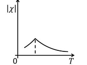
(P) Diamagnetic (2) 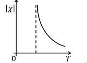
(Q) Paramagnetic (3) 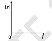
(R) Ferromagnetic (4) 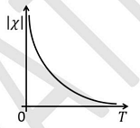
(S) Antiferromagnetic
Top GATE PH Mechanics Questions
- A paramagnetic material containing paramagnetic ions with total angular momentum \( J = \frac{1}{2} \) is kept at absolute temperature \( T \). The ratio of the magnetic field required for 80% of the ions to be in the lowest energy state to that required for having 60% of the ions to be in the lowest energy state at the same temperature is:
Consider a two-level system with energy states \( +\epsilon \) and \( -\epsilon \). The number of particles at \( +\epsilon \) level is \( N+ \) and the number of particles at \( -\epsilon \) level is \( N- \). The total energy of the system is \( E \) and the total number of particles is \( N = N+ + N- \). In the thermodynamic limit, the inverse of the absolute temperature of the system is:
(Given: \( \ln N! \approx N \ln N - N \))A two-level quantum system has energy eigenvalues \( E_1 \) and \( E_2 \). A perturbing potential \( H' = \lambda \Delta \sigma_x \) is introduced, where \( \Delta \) is a constant having dimensions of energy, \( \lambda \) is a small dimensionless parameter, and \( \sigma_x = \begin{pmatrix} 0 & 1 \\ 1 & 0 \end{pmatrix} \).
The magnitudes of the first and the second order corrections to \( E_1 \) due to \( H' \), respectively, are:- The energy of a free, relativistic particle of rest mass \( m \) moving along the \( x \)-axis in one dimension, is denoted by \( T \). When moving in a given potential \( V(x) \), its Hamiltonian is \( H = T + V(x) \). In the presence of this potential, its speed is \( v \), conjugate momentum \( p \), and the Lagrangian \( L \). Then, which of the following option(s) is/are correct?
- The Hamiltonian for a one-dimensional system with mass \( m \), position \( q \), and momentum \( p \) is: \[ H(p, q) = \frac{p^2}{2m} + q^2 A(q) \] where \( A(q) \) is a real function of \( q \). If \[ m \frac{d^2 q}{dt^2} = -5q A(q), \] then \[ \frac{d A(q)}{d q} = n \frac{A(q)}{q}. \] The value of \( n \) (in integer) is:
Top GATE PH Questions
- If \( F_1(Q, q) = Qq \) is the generating function of a canonical transformation from \((p, q)\) to \((P, Q)\), then which one of the following relations is correct?
- When an unpolarized plane electromagnetic wave in a dielectric medium with refractive index \( n_1 \) is incident on a plane interface separating it from another dielectric medium with refractive index \( n_2 \) (where \( n_2 > n_1 \)), and the angle of incidence is \(\tan^{-1} \left( \frac{n_2}{n_1} \right) \), the following statement is true:
- The wavefunction of a particle in an infinite one-dimensional potential well at time \( t \) is
\[ \Psi(x, t) = \sqrt{\frac{2}{3}} e^{-iE_1 t/\hbar}\psi_1(x) + \frac{1}{\sqrt{6}} e^{i\pi/6} e^{-iE_2 t/\hbar} \psi_2(x) + \frac{1}{\sqrt{6}} e^{i\pi/4} e^{-iE_3 t/\hbar} \psi_3(x) \]where \(\psi_1\), \(\psi_2\), and \(\psi_3\) are the normalized ground state, the normalized first excited state, and the normalized second excited state, respectively. \(E_1\), \(E_2\), and \(E_3\) are the eigen-energies corresponding to \(\psi_1\), \(\psi_2\), and \(\psi_3\), respectively. The expectation value of energy of the particle in state \(\Psi(x,t)\) is - If a thermodynamical system is adiabatically isolated and experiences a change in volume under an externally applied constant pressure, then the thermodynamical potential minimized at equilibrium is the
- The mean distance between the two atoms of an HD molecule is \( r \), where H and D denote hydrogen and deuterium, respectively. The mass of the hydrogen atom is \( m_H \). The energy difference between the two lowest lying rotational states of HD in multiples of \(\frac{h^2}{m_H r^2}\) is: